Data types & Vectors & Pivoting

Research Beyond the Lab: Open Science and Research Methods for a Global Engineer

Lars Schöbitz

2024-03-28

Course calendar

• 04th April 2024: no class, Easter Break

module	date	topic
1	22 February 2024	Welcome & get ready for the course
2	29 February 2024	Data science lifecycle & Exploratory data analysis using visualization
3	07 March 2024	Data transformation with dplyr
4	14 March 2024	Data import & Data organization in spreadsheets
5	21 March 2024	Conditions & Dates & Tables
6	28 March 2024	Data types & Vectors & Pivoting
NA	04 April 2024	Easter Break
7	11 April 2024	Joining tables & Creating and publishing scholarly articles with Quarto and GitHub pages
8	18 April 2024	Waste Research
9	25 April 2024	Research Design
10	02 May 2024	Survey Design
NA	09 May 2024	Auffahrt Break
11	16 May 2024	Pre-test and logistics
NA	23 May 2024	Data collection
12	30 May 2024	Data analysis & report writing
NA	06 June 2024	Project Submission Deadline
NA	13 June 2024	Exam

Learning Objectives (for this week)

1. Learners can identify different ways of accessing a vector from a dataframe
2. Learners can list the four main atomic vector types in R.
3. Learners can apply functions from the tidyr R Package to transform their data from a wide to a long format and vice versa.

Part 1: Cross-references

Cross references

• Help readers to navigate your document with numbered references and hyperlinks to entities like figures and tables.

• Cross referencing steps:

  • Add a caption to your figure or table.
  • Give an ID to your figure or table, starting with fig- or tbl-.
  • Refer to it with @fig-... or @tbl-....

Table cross references

The presence of the caption (A few penguins) and label (#tbl-penguins) make this table reference-able:

See @tbl-penguins for data on a few penguins.

becomes:

See Table 1 for data on a few penguins.

```{r}
#| label: tbl-penguins
#| tbl-cap: A few penguins

head(penguins) |> 
  gt()
```

Table 1: A few penguins

species	island	bill_length_mm	bill_depth_mm	flipper_length_mm	body_mass_g	sex	year
Adelie	Torgersen	39.1	18.7	181	3750	male	2007
Adelie	Torgersen	39.5	17.4	186	3800	female	2007
Adelie	Torgersen	40.3	18.0	195	3250	female	2007
Adelie	Torgersen	NA	NA	NA	NA	NA	2007
Adelie	Torgersen	36.7	19.3	193	3450	female	2007
Adelie	Torgersen	39.3	20.6	190	3650	male	2007

Figure cross references

The presence of the caption (A few penguins) and label (#fig-penguins) make this figure reference-able:

See @fig-penguins for data on a few penguins.

becomes:

See Figure 1 for data on a few penguins.

```{r}
#| label: fig-penguins
#| fig-cap: A few penguins
#| fig-width: 6
#| fig-asp: 0.618

ggplot(penguins, aes(x = species, fill = species)) +
  geom_bar(show.legend = FALSE)
```

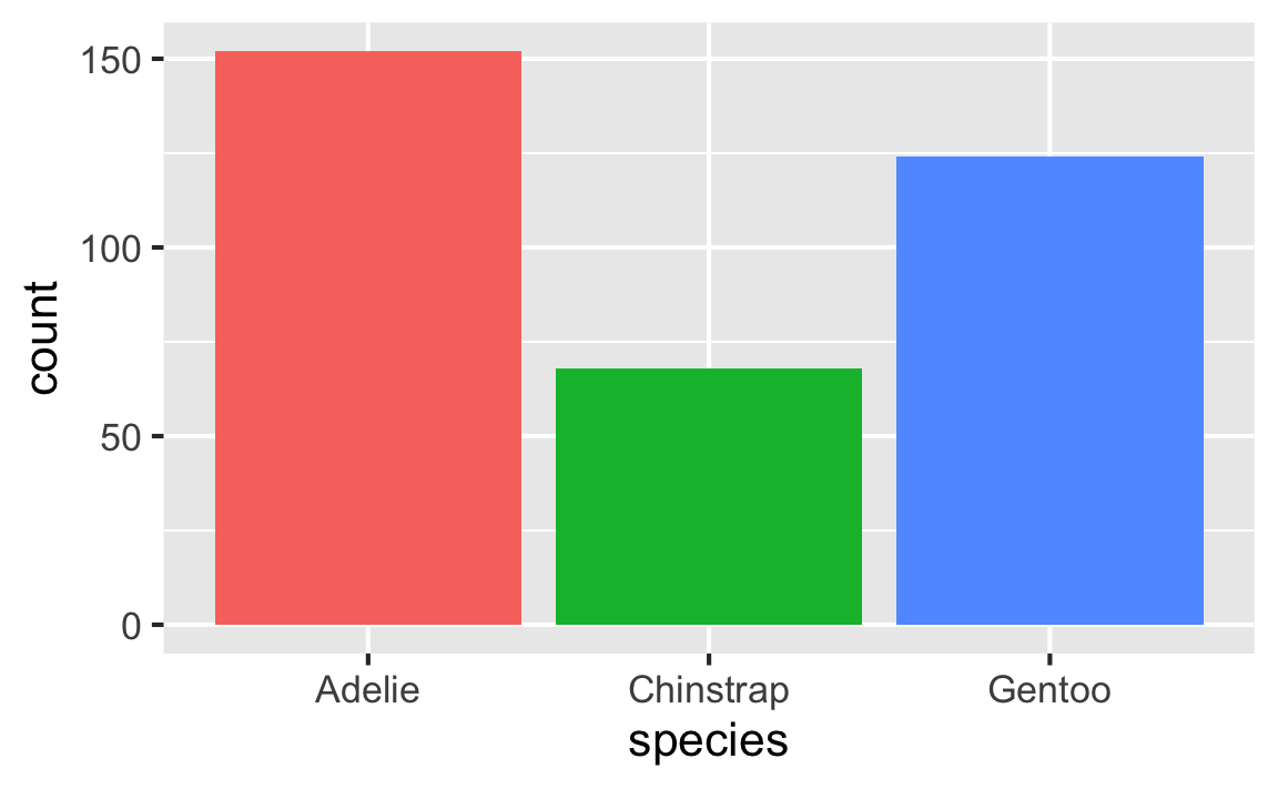
Figure 1: A few penguins

Your turn: md-06-exercises - cross-references

1. Open posit.cloud in your browser (use your bookmark).
2. Open the ds4owd workspace for the course.
3. In the File Manager in the bottom right window, locate the md-06a-cross-references.qmd file and click on it to open it in the top left window.
4. Follow instructions in the file

10:00

Part 2: Data types and vectors

Why care about data types?

via GIPHY

Example: survey data

A survey about recycling behaviour in the city of Zurich:

• job: What is your occupation?
• price_glass: What monthly subscription would you be willing to pay for a metal/glass bin outside your home?

id	job	price_glass
1	Student	0
2	Retired	0
3	Other	0
4	Employed	10
5	Employed	See comment
6	Student	5-10
7	Student	0
8	Retired	0
9	Student	10
10	Employed	0
11	Employed	20 (2chf per person with 10 people in the WG)
12	Student	10
13	Student	10
14	Employed	0
15	Student	10
16	Student	0
17	Employed	5-10
18	Other	0
19	Student	0
20	Employed	10
21	Employed	0
22	Employed	5

Oh why won’t you work?!

survey_data_small |> 
  summarise(mean_price_glass = mean(price_glass))

# A tibble: 1 × 1
  mean_price_glass
             <dbl>
1               NA

Oh why won’t you still work??!!

survey_data_small |> 
  summarise(mean_price_glass = mean(price_glass, na.rm = TRUE))

# A tibble: 1 × 1
  mean_price_glass
             <dbl>
1               NA

Take a breath and look at your data

id	job	price_glass
1	Student	0
2	Retired	0
3	Other	0
4	Employed	10
5	Employed	See comment
6	Student	5-10
7	Student	0
8	Retired	0
9	Student	10
10	Employed	0
11	Employed	20 (2chf per person with 10 people in the WG)
12	Student	10
13	Student	10
14	Employed	0
15	Student	10
16	Student	0
17	Employed	5-10
18	Other	0
19	Student	0
20	Employed	10
21	Employed	0
22	Employed	5

Take a breath and look at your data

# A tibble: 22 × 3
      id job      price_glass
   <int> <chr>    <chr>      
 1     1 Student  0          
 2     2 Retired  0          
 3     3 Other    0          
 4     4 Employed 10         
 5     5 Employed See comment
 6     6 Student  5-10       
 7     7 Student  0          
 8     8 Retired  0          
 9     9 Student  10         
10    10 Employed 0          
# ℹ 12 more rows

Very common data tidying step!

survey_data_small |> 
  mutate(price_glass_new = case_when(
    price_glass == "5-10" ~ "7.5",
    price_glass == "05-Oct" ~ "7.5",
    str_detect(price_glass, pattern = "2chf") == TRUE ~ "20",
    str_detect(price_glass, pattern = "See comment") == TRUE ~ NA_character_,
    TRUE ~ price_glass
  )) 

Very common data tidying step!

id	job	price_glass_new	price_glass
1	Student	0	0
2	Retired	0	0
3	Other	0	0
4	Employed	10	10
5	Employed	NA	See comment
6	Student	7.5	5-10
7	Student	0	0
8	Retired	0	0
9	Student	10	10
10	Employed	0	0
11	Employed	20	20 (2chf per person with 10 people in the WG)
12	Student	10	10
13	Student	10	10
14	Employed	0	0
15	Student	10	10
16	Student	0	0
17	Employed	7.5	5-10
18	Other	0	0
19	Student	0	0
20	Employed	10	10
21	Employed	0	0
22	Employed	5	5

Sumamrise? Argh!!!!

survey_data_small |> 
  mutate(price_glass_new = case_when(
    price_glass == "5-10" ~ "7.5",
    price_glass == "05-Oct" ~ "7.5",
    str_detect(price_glass, pattern = "20") == TRUE ~ "20",
    str_detect(price_glass, pattern = "See comment") == TRUE ~ NA_character_,
    TRUE ~ price_glass
  )) |> 
  summarise(mean_price_glass = mean(price_glass_new, na.rm = TRUE))

# A tibble: 1 × 1
  mean_price_glass
             <dbl>
1               NA

Always respect your data types!

Taking the mean of vector with type “character” is not possible.

# A tibble: 22 × 4
      id job      price_glass price_glass_new
   <int> <chr>    <chr>       <chr>          
 1     1 Student  0           0              
 2     2 Retired  0           0              
 3     3 Other    0           0              
 4     4 Employed 10          10             
 5     5 Employed See comment <NA>           
 6     6 Student  5-10        7.5            
 7     7 Student  0           0              
 8     8 Retired  0           0              
 9     9 Student  10          10             
10    10 Employed 0           0              
# ℹ 12 more rows

Always respect your data types!

survey_data_small |> 
  mutate(price_glass_new = case_when(
    price_glass == "5-10" ~ "7.5",
    price_glass == "05-Oct" ~ "7.5",
    str_detect(price_glass, pattern = "20") == TRUE ~ "20",
    str_detect(price_glass, pattern = "See comment") == TRUE ~ NA_character_,
    TRUE ~ price_glass
  )) |> 
  mutate(price_glass_new = as.numeric(price_glass_new)) |> 
  summarise(mean_price_glass = mean(price_glass_new, na.rm = TRUE))

# A tibble: 1 × 1
  mean_price_glass
             <dbl>
1             4.76

My turn: Types of vectors & For loops

Sit back and enjoy!

25:00

Take a break

Please get up and move! Let your emails rest in peace.

10:00

Your turn: md-06-exercises - types

1. Open posit.cloud in your browser (use your bookmark).
2. Open the ds4owd workspace for the course.
3. In the File Manager in the bottom right window, locate the md-06b-types-your-turn.qmd file and click on it to open it in the top left window.
4. Follow instructions in the file

35:00

Take a break

Please get up and move! Let your emails rest in peace.

10:00

Part 3: tidyr - long and wide formats

.

Illustrations from the Openscapes blog Tidy Data for reproducibility, efficiency, and collaboration by Julia Lowndes and Allison Horst

.

Illustrations from the Openscapes blog Tidy Data for reproducibility, efficiency, and collaboration by Julia Lowndes and Allison Horst

.

Illustrations from the Openscapes blog Tidy Data for reproducibility, efficiency, and collaboration by Julia Lowndes and Allison Horst

A grammar of data tidying

The goal of tidyr is to help you tidy your data via

• pivoting for going between wide and long data
• splitting and combining character columns
• nesting and unnesting columns
• clarifying how NAs should be treated

Slide taken from Data Science in a Box

Pivoting data

Waste characterisation data

objid	location	pet	metal_alu	glass	paper	other	total
900	eth	0.06	0.06	0.58	0.21	1.14	2.05
899	eth	0.14	0.01	0.18	0.28	3.04	3.64
921	old_town	0.00	0.00	0.00	0.41	1.57	1.99
916	old_town	0.17	0.04	0.80	0.55	0.62	2.19
900	eth	0.10	0.04	0.00	0.40	0.58	1.12
899	eth	0.08	0.03	0.00	0.05	0.34	0.50
921	old_town	0.08	0.03	0.30	0.40	1.52	2.33
916	old_town	0.11	0.04	0.92	1.01	1.99	4.07

How would you plot this?

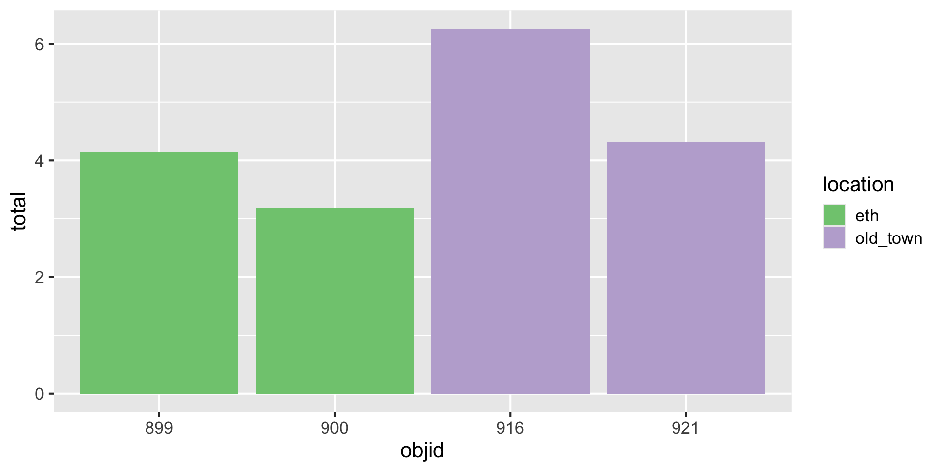
Three variables

objid	location	total
900	eth	2.05
899	eth	3.64
921	old_town	1.99
916	old_town	2.19
900	eth	1.12
899	eth	0.50
921	old_town	2.33
916	old_town	4.07

Three variables -> three aesthetics

ggplot(data = waste_data_untidy,
       mapping = aes(x = objid, 
                     y = total, 
                     fill = location)) +
  geom_col() + 
  scale_fill_brewer(type = "qual")

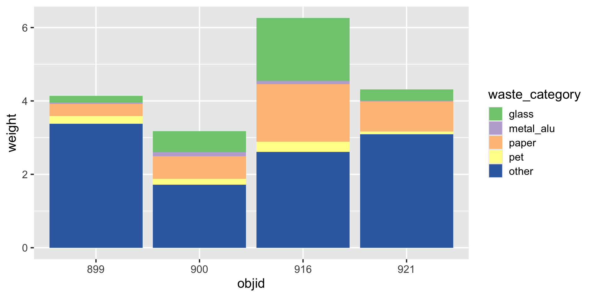
And how to plot this?

Reminder: Data (in wide format)

objid	location	pet	metal_alu	glass	paper	other
900	eth	0.06	0.06	0.58	0.21	1.14
899	eth	0.14	0.01	0.18	0.28	3.04
921	old_town	0.00	0.00	0.00	0.41	1.57
916	old_town	0.17	0.04	0.80	0.55	0.62
900	eth	0.10	0.04	0.00	0.40	0.58
899	eth	0.08	0.03	0.00	0.05	0.34
921	old_town	0.08	0.03	0.30	0.40	1.52
916	old_town	0.11	0.04	0.92	1.01	1.99

You need: A long format

objid	location	waste_category	weight
900	eth	pet	0.06
900	eth	metal_alu	0.06
900	eth	glass	0.58
900	eth	paper	0.21
900	eth	other	1.14
899	eth	pet	0.14
899	eth	metal_alu	0.01
899	eth	glass	0.18
899	eth	paper	0.28
899	eth	other	3.04
921	old_town	pet	0.00
921	old_town	metal_alu	0.00
921	old_town	glass	0.00
921	old_town	paper	0.41
921	old_town	other	1.57
916	old_town	pet	0.17
916	old_town	metal_alu	0.04
916	old_town	glass	0.80
916	old_town	paper	0.55
916	old_town	other	0.62
900	eth	pet	0.10
900	eth	metal_alu	0.04
900	eth	glass	0.00
900	eth	paper	0.40
900	eth	other	0.58
899	eth	pet	0.08
899	eth	metal_alu	0.03
899	eth	glass	0.00
899	eth	paper	0.05
899	eth	other	0.34
921	old_town	pet	0.08
921	old_town	metal_alu	0.03
921	old_town	glass	0.30
921	old_town	paper	0.40
921	old_town	other	1.52
916	old_town	pet	0.11
916	old_town	metal_alu	0.04
916	old_town	glass	0.92
916	old_town	paper	1.01
916	old_town	other	1.99

Three variables -> three aesthetics

ggplot(data = waste_data_tidy,
       mapping = aes(x = objid, 
                     y = weight, 
                     fill = waste_category)) +
  geom_col() + 
  scale_fill_brewer(type = "qual")

How to

waste_data_untidy 

objid	location	pet	metal_alu	glass	paper	other
900	eth	0.06	0.06	0.58	0.21	1.14
899	eth	0.14	0.01	0.18	0.28	3.04
921	old_town	0.00	0.00	0.00	0.41	1.57
916	old_town	0.17	0.04	0.80	0.55	0.62
900	eth	0.10	0.04	0.00	0.40	0.58
899	eth	0.08	0.03	0.00	0.05	0.34
921	old_town	0.08	0.03	0.30	0.40	1.52
916	old_town	0.11	0.04	0.92	1.01	1.99

How to

waste_data_untidy |> 
  pivot_longer(cols = pet:other,
               names_to = "waste_category",
               values_to = "weight") 

objid	location	waste_category	weight
900	eth	pet	0.06
900	eth	metal_alu	0.06
900	eth	glass	0.58
900	eth	paper	0.21
900	eth	other	1.14
899	eth	pet	0.14
899	eth	metal_alu	0.01
899	eth	glass	0.18
899	eth	paper	0.28
899	eth	other	3.04
921	old_town	pet	0.00
921	old_town	metal_alu	0.00
921	old_town	glass	0.00
921	old_town	paper	0.41
921	old_town	other	1.57
916	old_town	pet	0.17
916	old_town	metal_alu	0.04
916	old_town	glass	0.80
916	old_town	paper	0.55
916	old_town	other	0.62
900	eth	pet	0.10
900	eth	metal_alu	0.04
900	eth	glass	0.00
900	eth	paper	0.40
900	eth	other	0.58
899	eth	pet	0.08
899	eth	metal_alu	0.03
899	eth	glass	0.00
899	eth	paper	0.05
899	eth	other	0.34
921	old_town	pet	0.08
921	old_town	metal_alu	0.03
921	old_town	glass	0.30
921	old_town	paper	0.40
921	old_town	other	1.52
916	old_town	pet	0.11
916	old_town	metal_alu	0.04
916	old_town	glass	0.92
916	old_town	paper	1.01
916	old_town	other	1.99

Three variables -> three aesthetics

ggplot(data = waste_data_tidy,
       mapping = aes(x = objid, 
                     y = weight, 
                     fill = waste_category)) +
  geom_col() + 
  scale_fill_brewer(type = "qual")

Homework assignments module 6

Module 6 documentation

rbtl-fs24.github.io/website/modules/md-06.html

Homework due date

• Homework assignment due: Wednesday, April 10th

Wrap-up

Thanks! 🌻

Slides created via revealjs and Quarto: https://quarto.org/docs/presentations/revealjs/ Access slides as PDF on GitHub

All material is licensed under Creative Commons Attribution Share Alike 4.0 International.

References

Ben Aleya, Ali, Daniel Biek, Lin Boynton, Julia Jaeggi, Sebastian Camilo Loos, Chiara Meyer-Piening, Jonathan Olal Ogwang, et al. 2022. “Research Beyond the Lab, Spring Term 2022, Global Health Engineering, ETH Zurich. Raw Data and Analysis-Ready Derived Data on Waste Management in Public Spaces in Zurich, Switzerland.” Zenodo. https://doi.org/10.5281/ZENODO.7331120.